For your application it may be more interesting to train an already trained machine learning model, for a different but related problem. We exploit what has been learned in one task to improve the performance in another. This is useful if for example we do not have much labeled data. Other advantages are reduced training time and better performance.
Here we will guide you through the steps required to train with transfer learning the model using a dataset as an example that could be useful for a Quality Control task in manufacturing, and the steps required to visualize, check if the model works and to deploy it for edge devices for on-premise inference.
Imports.
import itertools

import os

import matplotlib.pylab as plt

import numpy as np

import os

import tensorflow as tf

import tensorflow_hub as hub
Download model
If you want to do transfer learning, your starting point is an already trained model, you can obtain these from different repositories, we will use TensorFlow Hub.
Choose a SavedModel from the tensorflow hub, there are many models with different structures and amount of parameters and trained on different datasets. Get a link to use that particular model in your Python code. We will be using efficientnetv2 trained on the imagenet-21k dataset.
model_name = "efficientnetv2-xl-21k"

model_handle_map = {

    "efficientnetv2-xl-21k": "https://tfhub.dev/google/imagenet/efficientnet_v2_imagenet21k_xl/feature_vector/2"

}

model_handle = model_handle_map.get(model_name)

#Define the size according to the model specifications.

pixels = 512

IMAGE_SIZE = (pixels, pixels)

print(f"Input size {IMAGE_SIZE}")

#If you have gpu you can use a larger Batch size

BATCH_SIZE = 16
#Build the dataset.
We will use a dataset from kaggle for food inspection, containing two classes, one with fresh meat and the other with spoiled meat. This is just one example of the many applications we could use deep learning for quality assurance in manufacturing.
O.Ulucan , D.Karakaya and M.Turkan.(2019) Meat quality assessment based on deep learning. In Conf. Innovations Intell. Syst. Appli. (ASYU)
myFile= "Path/to/dataset.zip"

fullPath = os.path.abspath(myFile)

print(fullPath)

#We will train a model to assess meat quality.

data_for_processing =tf.keras.utils.get_file(origin='file://'+fullPath, extract=True)

def build_dataset(subset):

  return tf.keras.preprocessing.image_dataset_from_directory(

   "archive",

   validation_split=.20,

   subset=subset,

   label_mode="categorical",

   # Seed needs to provided when using validation_split and shuffle = True.

   # A fixed seed is used so that the validation set is stable across runs.

   seed=123,

   image_size=IMAGE_SIZE,

   batch_size=1)

train_ds = build_dataset("training")

class_names = tuple(train_ds.class_names)

train_size = train_ds.cardinality().numpy()

train_ds = train_ds.unbatch().batch(BATCH_SIZE)

train_ds = train_ds.repeat()

normalization_layer = tf.keras.layers.Rescaling(1. / 255)

preprocessing_model = tf.keras.Sequential([normalization_layer])

#You could add data_augmentation to obtain a larger dataset, #and the model will perform better overall

#Example:   preprocessing_model.add(

# tf.keras.layers.RandomTranslation(0.2, 0))

train_ds = train_ds.map(lambda images, labels:

                     (preprocessing_model(images), labels))

#Validation dataset

val_ds = build_dataset("validation")

valid_size = val_ds.cardinality().numpy()

val_ds = val_ds.unbatch().batch(BATCH_SIZE)

val_ds = val_ds.map(lambda images, labels:

                 (normalization_layer(images), labels))
Building the model.
Next, we will build the model layers, because we will be using an already training model we will freeze the parameters of the model and work on the output layer.
model = tf.keras.Sequential([

# Explicitly define the input shape so the model can be

# properly loaded by the TFLiteConverter

tf.keras.layers.InputLayer(input_shape=IMAGE_SIZE + (3,)),

hub.KerasLayer(model_handle, trainable=False),

tf.keras.layers.Dropout(rate=0.2),

tf.keras.layers.Dense(len(class_names),                      kernel_regularizer=tf.keras.regularizers.l2(0.0001))

])

model.build((None,)+IMAGE_SIZE+(3,))

model.summary()

model.compile(

  optimizer=tf.keras.optimizers.SGD(learning_rate=0.005, momentum=0.9),

  loss=tf.keras.losses.CategoricalCrossentropy(from_logits=True, label_smoothing=0.1),

  metrics=['accuracy'])
Training
Adjust the number of epochs according to the duration of the training, this will take you the longest, it is important to correctly choose the number of epochs to obtain a good performance but make sure not to get into overfitting territory.
steps_per_epoch = train_size // BATCH_SIZE

validation_steps = valid_size // BATCH_SIZE

hist = model.fit(

    train_ds,

    epochs=5, steps_per_epoch=steps_per_epoch,

    validation_data=val_ds,

    validation_steps=validation_steps).history
Statistics.
When training has finished, we would like to check how well we can expect our model to perform, the next plots can help us look at this. We will look at the values of our model’s loss and precision.
plt.figure()

plt.ylabel("Loss (training and validation)")

plt.xlabel("Training Steps")

plt.plot(hist["loss"])

plt.plot(hist["val_loss"])

plt.figure()

plt.ylabel("Accuracy (training and validation)")

plt.xlabel("Training Steps")

plt.ylim([0,1])

plt.plot(hist["accuracy"])

plt.plot(hist["val_accuracy"])

plt.savefig("res1.png")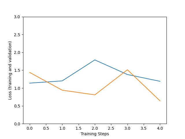
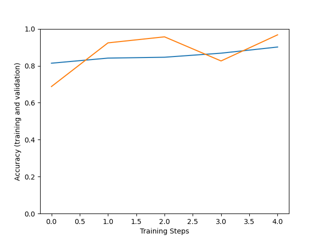
Improvement of the accuracy (number of correct guesses) and loss (difference between model output and expected values) is not linear. But the usual trend is that the larger the training steps the more fitting are the model predictions to our dataset, but be careful with overfitting.
Test on validation set.
We can perform inference on an image in the validation set. The model will return if the image provided is from the fresh or spoiled category.
x, y = next(iter(val_ds))

image = x[0, :, :, :]

true_index = np.argmax(y[0])

# Expand the validation image to (1, 224, 224, 3) before predicting the label

prediction_scores = model.predict(np.expand_dims(image, axis=0))

predicted_index = np.argmax(prediction_scores)

print("True label: " + class_names[true_index])

print("Predicted label: " + class_names[predicted_index])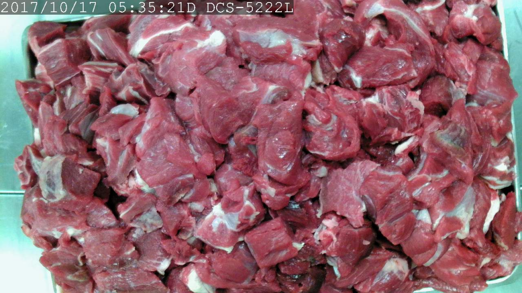
Predicted label: Fresh
Save the model.
Once the training has finished you can save your model with the parameters to be used on later applications.
tf.saved_model.save(model, saved_model_path)Export
Export model to tflite for use on Edge devices, for example raspberry, mobile phones or Google Coral.
It is possible to perform optimizations to the model for better performance on mobile devices, like quantizations.
lite_model_content = converter.convert()

with open(f"/tmp/lite_flowers_model_{model_name}.tflite", "wb") as f:

  f.write(lite_model_content)

print("Wrote %sTFLite model of %d bytes." %

   ("optimized " if optimize_lite_model else "", len(lite_model_content)))

interpreter = tf.lite.Interpreter(model_content=lite_model_content)

# This little helper wraps the TFLite Interpreter as a numpy-to-numpy function.

def lite_model(images):

  interpreter.allocate_tensors()

  interpreter.set_tensor(interpreter.get_input_details()[0]['index'], images)

  interpreter.invoke()

  return interpreter.get_tensor(interpreter.get_output_details()[0]['index'])

num_eval_examples = 50

eval_dataset = ((image, label)  # TFLite expects batch size 1.

                for batch in train_ds

                for (image, label) in zip(*batch))

count = 0

count_lite_tf_agree = 0

count_lite_correct = 0

for image, label in eval_dataset:

  probs_lite = lite_model(image[None, ...])[0]

  probs_tf = model(image[None, ...]).numpy()[0]

  y_lite = np.argmax(probs_lite)

  y_tf = np.argmax(probs_tf)

  y_true = np.argmax(label)

  count +=1

  if y_lite == y_tf: count_lite_tf_agree += 1

  if y_lite == y_true: count_lite_correct += 1

  if count >= num_eval_examples: break

print("TFLite model agrees with original model on %d of %d examples (%g%%)." %

      (count_lite_tf_agree, count, 100.0 * count_lite_tf_agree / count))

print("TFLite model is accurate on %d of %d examples (%g%%)." %

      (count_lite_correct, count, 100.0 * count_lite_correct / count))
When you have downloaded the model and have your label files ready, you can perform as many inferences as you want. Without the need to train your model again.
If you would like to use your model on Google Coral, you would need to copy your files to your coral sd image. You could do it with the help of a bash script to mount a Google Coral image on your Linux machine.
losetup -f /Path/to/image

//Look for the loop device where the virtual disk has been installed

if mount /dev/loopXX /media; then

   echo "Mounted"

else

   echo "Doesn't exist, losetup failed"

fi

cp -i  $modelo $labels /media/home/mendel/

umount -d /media/image-coral/
Now you only need to have an inference script inside your device to use your trained model, you could make use of the following script.
Inference
Finally, once we have our tflite model, you can perform the inference on your device with the following script, such as Coral or Raspberry. If you have a TPU make sure to enable it for better performance.
from tflite_runtime.interpreter import Interpreter

import numpy as np

import tensorflow as tf

from PIL import Image as ImagePIL

import time

from numpy import asarray, transpose, tri

from PIL import ImageTk

import tflite_runtime.interpreter as tflite

import pprint

import cv2

pp = pprint.PrettyPrinter(indent=4) # Set Pretty Print Indentation

model = "/path/to/.tflite"

labels_path = "/path/to/labels.txt"

img = "/path/to/image"

#load labels from ffile.

def load_labels(filename):

  with open(filename, 'r') as f:

return [line.strip() for line in f.readlines()]

labels = load_labels(labels_path)

#Model

global interpreter, input_details, output_details

interpreter = tflite.Interpreter(model)

interpreter.allocate_tensors()

#experimental_delegates=[tflite.load_delegate('libedgetpu.so.1')])

input_details = interpreter.get_input_details()

output_details = interpreter.get_output_details()

_, height, width, _ = interpreter.get_input_details()[0]['shape']

# print('tensor input', input_details)

global size

size = [width, height]

print(size)

inicio=time.time()

#Open the image

img = cv2.imread(img)

img_resized = cv2.resize(img, (224, 224))

input_data = np.array(asarray(img_resized), dtype=np.float32)

input_data = np.expand_dims(input_data , axis=0)

# check the type of the input tensor

floating_model = input_details[0]['dtype'] == np.float32

#floating_model = input_details[0]['dtype'] == np.float32

if floating_model:

  input_data = (np.float32(input_data) - 127.5) / 127.5

print("-> Input data:", input_data)

interpreter.set_tensor(input_details[0]['index'], input_data)

interpreter.invoke()

tensor_result= interpreter.get_tensor(output_details[0]['index'])[0]

print(tensor_result)

results = np.squeeze(tensor_result)

#[::-1] is a trick in python to obtain a list in the opposite order.

top_k= results.argsort()[-5:][::-1]

#We get the top 5 results

result=''

#print(top_k)

for i in top_k:

result+=('{:08.6f}: {}'.format(float(tensor_result[i]), labels[i]))+"\n"

result=result+"Inference time: "+str(time.time()-inicio)

#print(resultado, '\n')

resultado_max= result.partition('\n')[0]+'\n'+ result.split('\n')[-1]

#Get the time it took for the inference

fin = time.time()

print("Inference time:" , fin-inicio)

print(resultado_max)

print("\n",result)